IAR GNSS Models
GNSS Carrier Phase Ambiguity Resolution Models
The GNSS Model
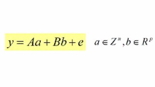
Every GNSS model can be cast in the following frame of linear(ized) observation equations:
with y the (incremental) vector of double differenced (DD) carrier-phase and pseudo range (code) observations, e its error vector, a de vector of unknown integer ambiguities, and b the vector of unknown baseline components and possibly other unknown real-valued parameters, such as atmospheric delays.
From float to fixed
Solving the GNSS model, implies finding ‘best’ estimates for the unknown parameter vectors a and b. Hereby one usually follows the following three steps.
Float solution
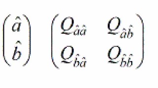
In the first step, the integerness of the ambiguities is discarded and the parameter vectors a and b are estimated by means of Least-Squares (LS). This gives
This solution is referred to as the ‘float solution’.
Integer solution
In the second step, an integer map S is defined, which maps the float ambiguity solution to an integer solution. Different choices for the integer map S are possible.
Fixed solution
This solution is referred to as the ‘float solution’.
In the final step, the integer ambiguity solution is used to correct the float baseline solution. This solution is referred to as the ‘fixed solution’.
If one may neglect the randomness of the integer ambiguity solution, the fixed baseline solution will have a much higher quality than the float baseline solution. To achieve this, is the whole purpose of GNSS carrier phase ambiguity resolution!
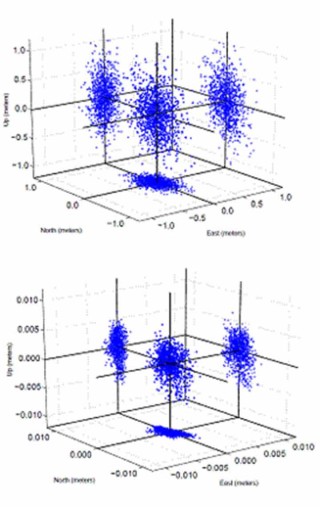
This improvement is demonstrated by the following two scatter plots. The scatter plot on the left is that of the float baseline, whereas the scatter plot on the right is that of the fixed baseline. Note the two orders of magnitude improvement. As the float solution is dominated by the code data and the fixed solution by the phase data, this improvement corresponds with the square-root of the phase-code variance ratio.