IAR Methods

Methods of Integer Ambiguity Resolution

There are many different ways for computing integer ambiguities from the real-valued float ambiguities. The three most popular methods are: (1) integer rounding, (2) integer bootstrapping, and (3) integer least-squares.

Integer rounding

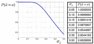
This method is the simplest of all. In this case the integer ambiguity solution is obtained from a component-wise nearest integer rounding of the float ambiguity vector. Integer rounding may be used if its probability of correct integer estimation, referred to as success-rate, is sufficiently close to 1. The success-rate depends on the precision of the float solution; the more precise the float solution, the higher the success-rate. The following graph and table show how, for the scalar case, the success-rate of rounding depends on the ambiguity standard deviation. To obtain a success-rate of 99.9%, a standard deviation of about 0.15 cycles is needed.

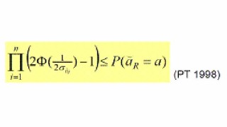
Computing the rounding success-rate is not that easy anymore in the vectorial case. In that case one can resort to simulation or make use of the lower bound.

For computing the lower bound, only the ambiguity standard deviations are needed.

Integer bootstrapping

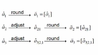
This method is a combination of integer rounding and sequential conditional least-squares estimation. Before a component of the float ambiguity solution is rounded, it is first adjusted following the integer values of its previous components:

Instead of the standard deviations, one now needs the conditional standard deviations as input for the success-rate computation. These conditional standard deviations are the square-roots of the nonzero entries of the diagonal matrix of the ambiguity variance matrix’ LDU-decomposition.
Bootstrapping is better than rounding, since it can be shown that the bootstrapped success-rate is never smaller than the rounding success-rate (PT 1998).

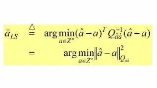
Integer least-squares

This method uses all the entries of the ambiguity variance matrix and it is defined as follows,

This method provides the best integer estimator of all, since it can be shown to have the largest success-rate of all admissible integer estimators.

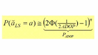
Simulation is used to compute the least-squares success-rate. Alternatively, one can make use of the easy-to-compute ADOP-based approximation.

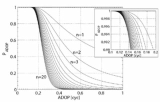
The ADOP (Ambiguity Dilution Of Precision) is defined as the determinant of the ambiguity variance matrix to the power 1/2n. It is a generalized ambiguity precision measure that has the important property of being invariant against ambiguity re-parametrization (PT 1997). The below graph shows the ADOP-based success-rate as function of the ADOP for varying n. It shows that for n ≤ 20, an ADOP of 0.12 cycles gives a success-rate better than 99.9%.

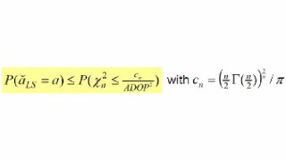
As an alternative to simulation or approximation, one may use bounds of the least-squares success-rate. The least-squares success-rate is bounded from below by the easy-to-compute bootstrapped success-rate and it is bounded from above as: